Noise Helps Signal Detection
Surface nuclear magnetic resonance (SNMR) is one of the most precious signals in the world of hydrogeophysics. Precious in terms of the information it contains, but also in its intrinsic fragility. The surface NMR signal is often swamped by interference from powerlines and even electromagnetic radiation from far off lightning storms. Even after many years, when I see a water signal in surface NMR measurement, I’m still in awe that it works.
The question is what are the limits on surface NMR ability to detect water? For a long time, I believed the answer depended on how finely we discretize our analogue signal; the resolution of the bit determines the smallest possible signal we can measure. My rational for this belief was that if the NMR signal is not large enough to change the value of the measured bit, we could not observe the oscillator nature of the NMR signal and therefore we would not detect its presence. If we take a noise-free signal, discretize it, if the signal amplitude is always below 1/2 the bit resolution, the digitized signal will be a stream of zeros. No detected signal. But, my supervisor, wisely postulated that the presence of noise means this is not the fundamental limit on a signal detectibility. This does not match my intuition. Can adding noise actually improve a signals detectibility? This is the inspiration for this post. Let’s look at some simulations.
To start we’ll check the noise-free case, discretizing a signal.
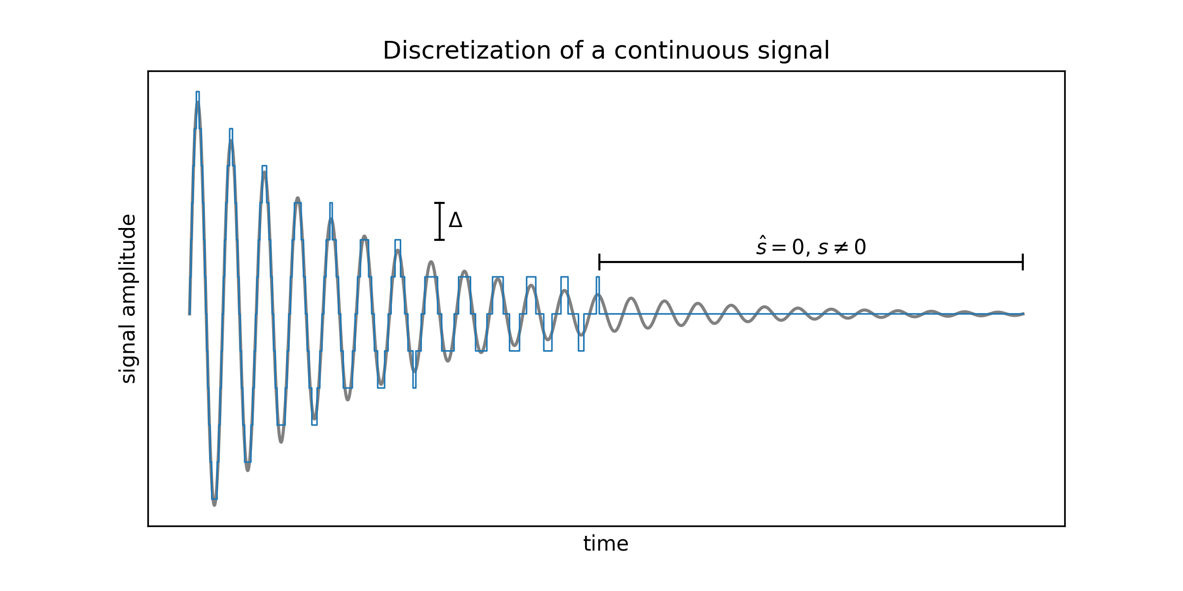
Figure 1: A discretized exponential decay.
In the background we see an idealized surface NMR signal; a single frequency oscillation with an exponentially decaying envelope. Setting the bit resolution to $\Delta$, we see the more staircase-like nature of the digitized signal in blue. Here we confirm our intuition; when the signal amplitude is always below 1/2 the bit resolution, the digitized signal is a stream of zeros. No detected signal for the second half of this noise-free recording.
With this illustration of the discretization process, lets look at signal detectibility. For this lets further simplify the process by considering a mono-frequency, sinusoidal signal. We’ll then use Fourier analysis ($\mathcal{F}$) via the Fast Fourier Transform (FFT) to investigate the detectibility of the signal.
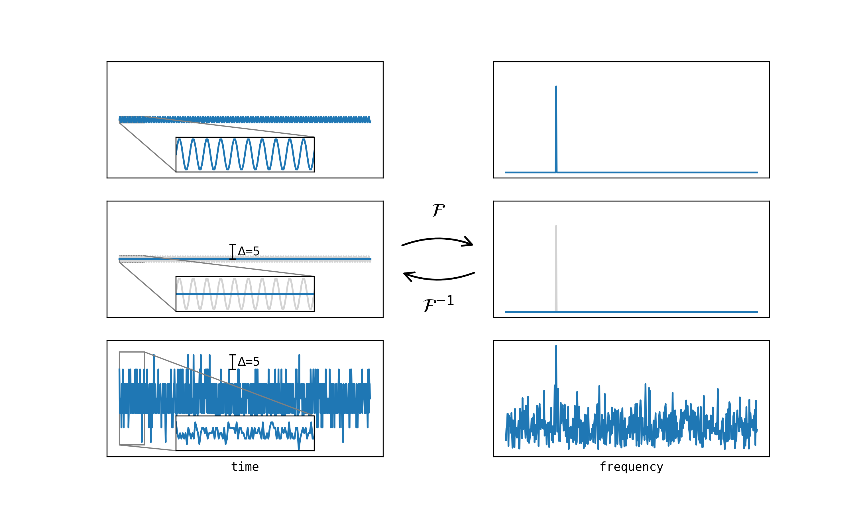
Figure 2: Fourier analysis of continous and discretized signals.
The top row shows the sinusoid along side its Fourier transform. Since it is a pure sinsoid, its frequency spectra is a single spike at the particular frequency. The middle row shows the discretized sinusoid; since the amplitude is below the resolution of the discretization, we round all the values to zero. Hence we see zeros in both time and frequency domain representations for this signal. Not surprising, following the example of the exponential of Figure 1. The final row, however, shows the pure sinusoid embedded in gaussian noise that has then been discretized. Even though the amplitude of the sinusoid is the same, adding the noise reveals a strong peak at the signal frequency in the frequency domain. In a sense the signal gets its head above the water by riding the random noise, and becomes detectable.
Of course, there are many parameters to play with here – signal amplitude, discretization level, and standard deviation of the noise for example – to see how robust this finding is. But this simple example illustrates something I find very counter-intuitive.
- sidenote: applying a window to a signal (for example, zeroing out the pulses) means that no matter what amplitudes are present in this interval, the result will be zero there. Looking at this in the frequency domain, the convolution with the window spectra still results in this zeroed interval in the time-domain.